The branch of Mathematics which deals with collection, classification and interpretation of data is called statistics.

When used in the singular sense, statistics refers to the subject as a whole of science of statistical methods embodying the theory and techniques. When it is used in the plural sense, statistics refers to the data itself (ie, numerical facts collected in a systematic manner with some definite purpose in view, in any field of enquiry).

The Frequency Table or the Frequency Distribution

If the data is classified in a convenient way and presented in a table it is called frequency table or frequency distribution.
Frequency: When the data is presented in a frequency table, the number of observations that fall in any particular class is called the frequency of that class.

Class Limit: The starting and end values of each class are called “lower limit” and “upper limit” of that class respectively.

Class-interval: The difference between the upper and lower boundary of a class is called the “class-interval” or “size of the class”. It can also be defined as the difference between the lower or upper limits or boundaries of two consecutive classes.

Class Boundaries: The average of the upper limit of a class and the lower limit of the succeeding class is called the “upper boundary” of that class. The upper boundary of a class becomes the “lower boundary” of the next class.

Range: The difference between the highest and the lowest observation of a data is called its range.

Histogram: Pertaining to a frequency distribution, if the true limits of the classes are taken on the x-axis and the corresponding frequencies on the y-axis and adjacent rectangles are drawn, the diagram is called ‘histogram’.

Frequency Polygon and Frequency Curve: If the points pertaining to the mid values of the classes of a frequency distribution and the corresponding frequencies are plotted on a graph sheet and these points are joined by straight lines, the figure formed is called frequency polygon. If these points are joined by a smooth curve the figure formed is called frequency curve.

Cumulative Frequency Curves: If the points pertaining to the boundaries of the classes of a frequency distribution and the corresponding cumulative frequencies are plotted on a graph sheet and they are joined by a smooth curve, the figure formed is called cumulative frequency curve. The figure formed with upper boundaries of the classes and the corresponding less than cumulative frequencies is called less than cumulative frequency curve. The figure formed with lower boundaries of the classes and the corresponding greater than cumulative frequencies is called greater than cumulative frequency curve.

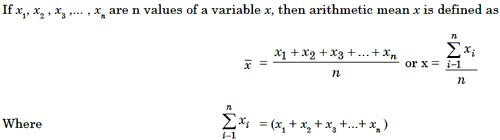
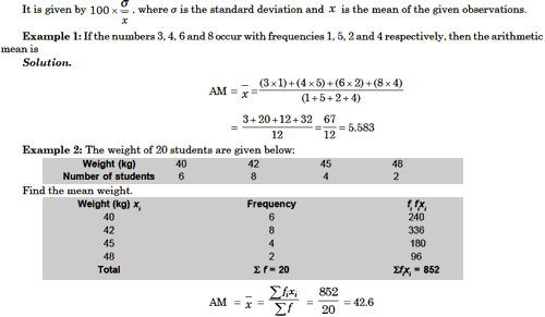
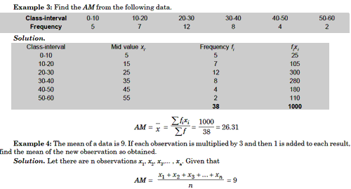
Arithmetic Mean (AM) or Mean

1. Arithmet ic Mean of Ungrouped Data

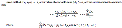
2. Arithmetic Mean of Grouped Data

Here, the mean may be computed by the following method

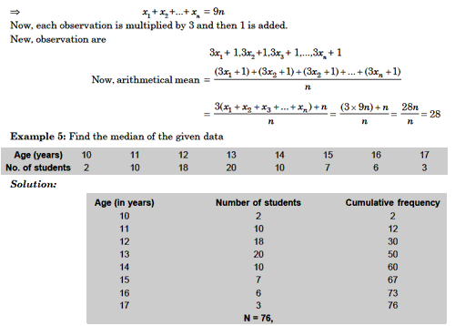
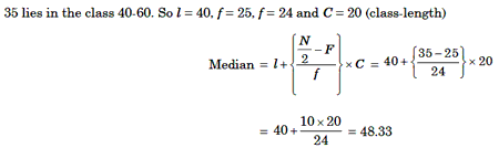
Median

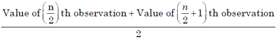
1. Median of Ungrouped Data If x1, x2, ... , xn are n values of variable x arranged in order of increasing or decreasing magnitude then the middle-most value in this arrangement is called the median.

If n is odd, then the median will be the n+1/2 th value arranged in order of magnitude. In this case there will be one and only one value of the median.

2. Median of Grouped Data

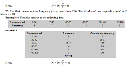
If N is the number of observation, we first calculate N/2 Then from the cumulative frequency distribution, we determine the class in which N/2 th observation lies. Let us name this as median class. We use the following formula for calculating the median.

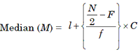
Where, l = lower boundary of the median class ie, the class where the N/2 TH observation lies.
N = total frequency
F = cumulative frequency of a class preceding the median class.
f = frequency of the median class.
C = length of the class interval.

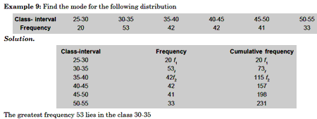
Mod e

The mode or modal value of a distribution is that value of the variable for which the frequency is maximum. For a given data, mode may or may not exist. If mode exists for a given data, it may or may not be unique. Data having unique mode is called uni-modal.While the data having two modes is called bi-modal.

1. Mode of Ungrouped Data

The observation with the highest frequency becomes the mode of the data.

2. Mode of Grouped Data

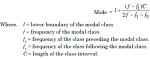
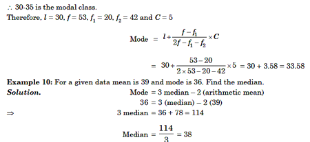
Relation between Mean, Median and Mode

3(Median) – 2(Mean) = Mode Measure of Dispersion
The dispersion of data is the measure of spreading (scatter) of the data about some central tendency. It is measured in the following types.
(a) Range
(b) Quartile Deviation
(c) Mean Deviation
(d) Standard Deviation
(e) Variance.

1. Range

Range is the difference of maximum and minimum values of the data. Range = Maximum value - Minimum value.

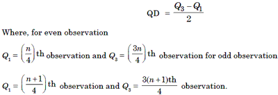
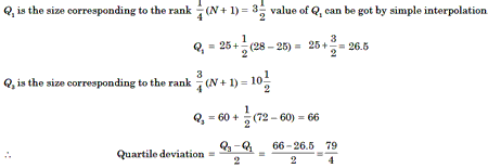
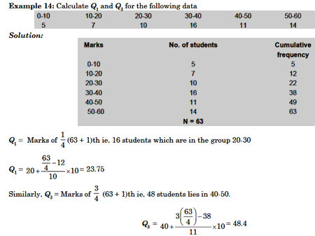
2. Quart i le Deviation

After arranging the data in the ascending order of magnitude we find

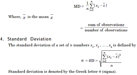
3. Mean Deviation

It is defined as the arithmetic mean of the absolute deviations of all the values taken about any central value. The mean deviation of a set of n numbers x₁, x₂, ... , x_n is defined by

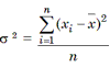
5. Variance

The variance of a set of it numbers x1, x2, ... , xn is defined as the square of the standard deviation.

6. Coefficient of Variation

Example 7: Find the range of marks of students in a class given as 60, 96, 28, 35, 10, 40, 9, 85, 25.
Solution. Maximum value = 96 Minimum value = 9 Range = Maximum value – Minimum value = 96 – 9 = 87

Example 8: Compute the quartile deviation from the following marks of 13 students in a class 25, 35, 9, 28, 52, 41, 38, 96, 85, 72, 10, 40, 60.
Solution. Let us arrange the given set of numbers in ascending magnitude. 9, 10, 25, 28, 35, 38, 40, 41, 52, 60, 72, 85, 96 Hence, N =13

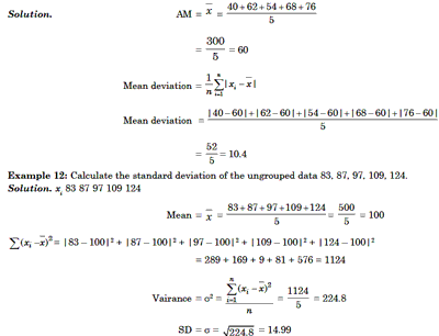
Example 11: Calculate the mean deviation of the variate 40, 62, 54, 68, 76.

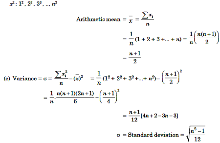
Example 13: Find the range, variance and standard deviation of the first n natural numbers.
Solution. Variable x takes the values 1, 2, 3, ..., n
(a) Range = n – 1
(b) x: 1, 2, 3,..., n

© UPSCPORTAL.COM